Summary of instructions to use the MCAL toolbox:
Purpose and Description: Model Calibration (MCAL) Toolbox is designed to perform Bayesian and approximate Bayesian analysis using Markov chain Monte Carlo simulation with differential evolution update. Formal Bayesian approach employs a traditional residual-based Gaussian likelihood function, and approximate Bayesian analysis allows for selection of one or multiple pre-specified summary statistic(s). The current version (as of 01/06/2017) of the toolbox only allows to choose among the provided conceptual rainfall runoff (RR) models (GR4J, GR5J, GR6J, HyMod, HBV, SACSMA). Future versions of MCAL will allow user to select any model (hydrologic or beyond) and any summary metric. Please contact mojtabasadegh@gmail.com if you need the flexible version.
How to Run:
Make sure to change the directory of matlab, to the directory that you saved the MCAL files in.
GUI:
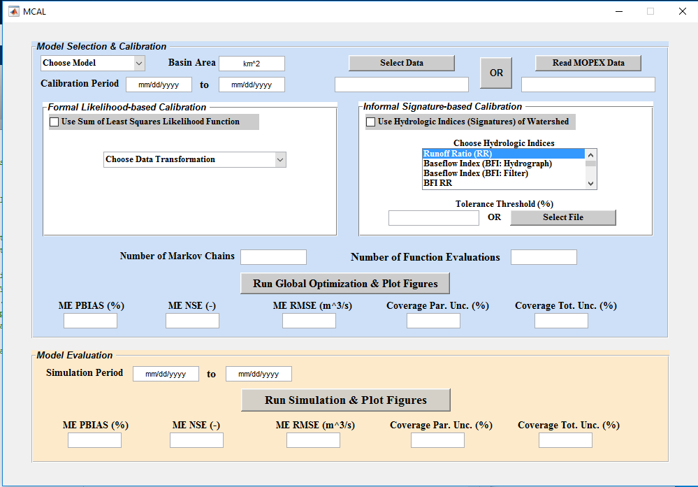
Run “MCAL.m” in matlab to open up the graphical user interface.
Calibration Step:
User is prompted to choose a CRR model (available models: GR4J, GR5J, GR6J, HyMod, HBV, SACSMA), calibration period (mm/dd/yyyy), basin area (km^2), and finally select observational data. User is allowed to load data in a “.txt” or “.dly” format, latter is the format of MOPEX data. Next step is to choose between formal Bayesian or approximate Bayesian approaches. If formal Bayesian approach is selected, user can also transform the data before performing the calibration. This option, however, is not yet activated (as of 01/06/2017) and will be added later. In this version the original observations will be used. If user opt to choose hydrologic indices for calibration of the RR model, then (s)he should select among the provided metrics (one or more). To select multiple metrics hold “ctrl” and click on any metric. Next step is to choose the tolerance threshold which is accepted in terms of percentage deviance from the observed metric (for example if the metric is 5 and threshold is 20, any simulation with metric of 4 (5-0.2*5) to 6 (5+0.2*5) will be accepted). If user needs to select different threshold value for each metric, it can be done by browsing a text file through “select file” button. Text file should not have any header and order of thresholds should be associated with order of selected metrics. Finally number of Markov chains and number of function evaluations should be inserted and then simulation should be run!
The MCAL toolbox will automatically create a graph with model simulation uncertainty ranges and observations and save the figure as “.png” to the “Results” folder. NSE, RMSE, percent bias performance metrics, as well as coverage of observations in the parameter uncertainty range and total uncertainty range (only in case of formal Bayesian) will also be reported to the user.
Analysis Step:
User should now select a simulation period and simply click on “Run Simulation & Plot Figures” and observe the results as graph and performance metrics on the screen. Plots will be saved as “.png” files in the “Results” folder.
Script:
Run the script “RUN_MCAL.m” in matlab after manually setting lines (33 or 41), 49, 55, 57, 61, 67, 70, 71, 78, and 81. Follow the comments in the script and instructions of GUI in this step.
Input:
Input file is either a text file (“.txt” format) with 8 columns of “year, month, day, precipitation, PET, streamflow, min temperature, max temperature” without any header; or be the “.dly” formatted data from MOPEX data set.
Outputs:
Parameter histograms and model simulation uncertainty ranges will be saved as “.png” figures in the “Results” folder. All the MCMC results are also saved as a “.mat” file in the “Results” folder.
Remarks:
User need to consider 365 days of spin up for any modeling using this toolbox.