Purpose and Description: Nonstationary Conceptual Rainfall Runoff Toolbox (NCRRT) is designed to allow for time variant modeling of rainfall runoff processes. It allows user to define one (and only one) parameter of the selected conceptual model (available models: GR4J, GR5J, GR6J, HyMod, HBV, SACSMA) time variant within any time interval to address the physical changes in the actual watershed. Time-variant parameter is changed linearly within the specified time interval, and can be defined as step change if the start and date of the interval are set identical. In this version (as of 01/05/2017) user should specify a calibration period (data set should allow for 365 days of spin up) that is assumed to be stationary (no changes in the properties of the watershed). This allows for estimation of model parameters by calibration against the available calibration data. Parameter estimation in this version is performed using a local optimization approach, in observation of the running time. We want this toolbox to be interactive and fast. It is assumed that these parameter value remain consistent for different time periods (might be violated, but pragmatic).
How to Run:
Make sure to change the directory of matlab, to the directory that you saved the NCRRT files in.
1. GUI: Run “NCRRT.m” in matlab to open up the graphical user interface.
Calibration Step:
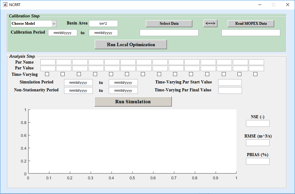
User is prompted to choose a CRR model (available models: GR4J, GR5J, GR6J, HyMod, HBV, SACSMA), calibration period (mm/dd/yyyy), basin area (km^2), and finally select observational data. User is allowed to load data in a “.txt” or “.dly” format, latter is the format of MOPEX data. When model is selected, model parameter names will automatically appear in the analysis step. After Calibration run is performed, parameter values will appear underneath parameter names. Also a plot will appear in the analysis step that shows model simulation vs observation in the calibration period. NSE, RMSE and percent bias performance metrics will also be reported to the user.
Analysis Step:
User should now interactively work with the toolbox to find parameter values that yield a good fit to the data observed in a nonstationary world. First is to check which parameter is time-varying (depends on the type of physical change in the real-world and definition of the parameters), then user should select a simulation period, as well as a period which is deemed as the time that non-stationarity has occurred. Next is to select the initial value for the time-varying parameter (usually set to the value obtained from calibration) and its final value. NCRRT automatically sets the parameter value before the start date of non-stationarity as initial value; and the parameter value after the non-stationarity period as the final value. Parameter value will linearly change in this period. User can now simply click on “Run Simulation” and observe the results as graph and performance metrics on the screen. This step is interactive and user should change the final time-varying parameter value until the desired result is obtained.
2. Script: Not provided for this toolbox!
Input:
Input file is either a text file (“.txt” format) with 8 columns of “year, month, day, precipitation, PET, streamflow, min temperature, max temperature” without any header; or be the “.dly” formatted data from MOPEX data set.
Outputs:
This is an interactive toolbox and results are shown on the screen within the GUI. Please see “Analysis Step” for more info.
Remarks:
User need to consider 365 days of spin up for any modeling using this toolbox.
Download NCRRT:
NCRRT_PCode (email mojtabasadegh@boisestate.edu to ask for .zip file)